
Imagine you’re a hiker exploring a vast, hilly landscape. As you hike, you’re climbing up and down various hills. After a while, you find yourself standing at the top of a particular hill. When you look around, you can see the landscape dipping down in all directions around you. Even if you take the smallest of steps forward, backward, to your left, or to your right, you start descending – the ground beneath you begins to slope downward.
In this situation, you’re standing at what we call a local maximum. The term “local” here implies that this is the highest point in your immediate vicinity or neighborhood. In terms of the function representing this landscape, the height of the hill you’re standing on is greater than the heights of the hills at any nearby point.
It’s important to note, however, that a local maximum is “local”. You may be standing at the highest point in your immediate vicinity, but when you look off into the distance, you may see higher peaks. Those higher peaks represent global maximum points – the absolute highest points across the entire landscape.
To understand the concept of a local maximum more intuitively, think about the smaller features of the landscape around you – little bumps, depressions, or hillocks on a bigger hill. Each of these features might have its local maximum – a point where, if you stand, every step leads downwards. But when you compare this point to the larger landscape, it’s not the absolute highest point.
This is why we use the term “local” – it’s all about the immediate surroundings of a point. It gives us a way to talk about the highs and lows of a function within a limited area, without having to take into account the whole function or landscape.
Look out for plateaus: Not all local maximums are pointed peaks; some might be flat spots or plateaus. Suppose you’re walking on a hill that levels out into a flat area. Everywhere you step within this flat area, the ground stays the same height. But as soon as you step off this flat area, you start going downhill. Even though the ground beneath you on the plateau isn’t rising or falling, you’re still at a local maximum. That’s because within your immediate vicinity, there are no higher points than the plateau. It’s only when you leave that immediate area that you find lower points, and possibly even higher points elsewhere. This example illustrates that a local maximum doesn’t have to be the very highest point overall; it’s about being higher than the points immediately surrounding it.
**Being in a valley:** Picture yourself standing in a vast valley surrounded by towering mountain peaks. You’re not on any of these peaks; instead, you’re standing atop a small mound of earth within the valley itself.
From the viewpoint of an observer flying high above the landscape, your position might not seem particularly impressive compared to the grandeur of the surrounding mountains. However, from your vantage point, things look different. As far as you can tell, within your immediate vicinity, you’re standing at the highest point. If you were to take a step in any direction—north, south, east, or west—you would descend from your mound, stepping down onto the lower valley floor.
Despite being surrounded by taller mountains, you are, in fact, at a local maximum. Your mound is the highest point in the local area, even though much higher points (the mountain peaks) exist beyond that local vicinity. This highlights the ‘local’ aspect of a local maximum—it’s not about being the highest point overall, but rather being higher than the points immediately surrounding it in a specific local region.
To emphasize, the concept of a local maximum does not necessarily mean you’re standing at the absolute highest point on the landscape. Instead, it means that within a specific, limited area, you are at the highest point, and any movement away from this point will lead you downwards.
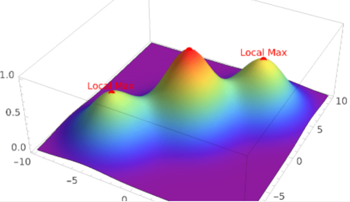
- \(e^{-0.1(x^{2} + y^{2})}\): This part of the function represents a Gaussian function (or bell curve) centered at the origin (0,0). The height of the peak is 1 (the coefficient in front of the Gaussian), and the spread or width of the peak is determined by the coefficient 0.1 in the exponent.
- \(0.7e^{-0.1((x – 5)^{2} + (y – 5)^{2})}\): This part of the function represents another Gaussian function centered at (5,5). The height of the peak is 0.7, and the spread is also determined by the coefficient 0.1 in the exponent.
- \(0.6e^{-0.1((x + 5)^{2} + (y + 5)^{2})}\): This part of the function represents a third Gaussian function centered at (-5,-5). The height of the peak is 0.6, and the spread is again determined by the coefficient 0.1 in the exponent.