Understanding the Midpoint Rule
The Midpoint Rule is a numerical method used to approximate the value of a definite integral. It provides a way to estimate the area under a curve, which is particularly useful when the integral cannot be calculated directly.
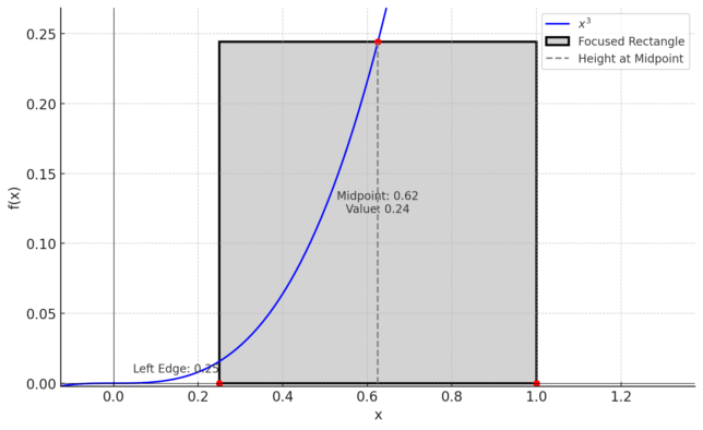
Why use midpoints? The idea is to improve the approximation’s accuracy. By taking the midpoint of each interval, we’re calculating the function’s value at a point that represents the average of the interval’s endpoints. This tends to give a better estimate of the area under the curve for that segment compared to using the endpoints or any other single point within the interval.
Sample Calculation:
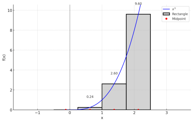
Let’s approximate the integral of x³ from -0.5 to 2.5 using 4 rectangles (n = 4).
- Calculate the width of each rectangle (Δx):
Δx = (2.5 – (-0.5)) / 4 = 0.75 - Determine the midpoints for each interval:
To find a midpoint, we start at the left endpoint of the interval and add half of Δx. This process is repeated for each interval:- x₀ = -0.5 + 0.75/2 = -0.125
- x₁ = -0.125 + 0.75 = 0.625
- x₂ = 0.625 + 0.75 = 1.375
- x₃ = 1.375 + 0.75 = 2.125
- Evaluate the function at each midpoint and sum the areas:
The function values at the midpoints are calculated and multiplied by Δx (the width of each rectangle), then summed to approximate the total area under the curve:- Area ≈ Δx [f(x₀) + f(x₁) + f(x₂) + f(x₃)]
- Area ≈ 0.75 [(-0.125)³ + (0.625)³ + (1.375)³ + (2.125)³]
- Area ≈ 9.31494140625
This calculated area, 9.31494140625, is the approximation of the integral using the Midpoint Rule.