The geometric series ∑ xⁿ from n=0 to ∞ has different behaviors depending on the value of x. For -1 < x < 1, the series converges, and the sum is given by 1 / (1 - x). When x = 1, the series 1 + 1 + 1 + ... diverges, and there is no finite sum. When x = -1, the series 1 - 1 + 1 - 1 + ... also diverges, and the sum does not converge to a finite value. These special cases illustrate the importance of the condition -1 < x < 1 for the sum formula to be valid.
Understanding the Sum of \( x^n \): A Geometric Series
A geometric series is a sequence of numbers where each term after the first is found by multiplying the previous term by a fixed number called the common ratio. In this case, the common ratio is \( x \), and the series can be expressed using sigma notation:
\( S = \sum_{n=0}^{\infty} x^n = 1 + x + x^2 + x^3 + \ldots \)
This series represents a pattern where you start with 1 and then multiply by \( x \) again and again, adding up all the terms.
Finding the Sum
If the common ratio \( x \) is between -1 and 1 (excluding -1 and 1), the terms get smaller and smaller, and the sum approaches a specific value. We can find this value using a clever trick:
1. Let \( S \) be the sum of the series: \( S = 1 + x + x^2 + x^3 + \ldots \)
2. Multiply both sides by \( x \): \( xS = x + x^2 + x^3 + x^4 + \ldots \)
3. Subtract the second equation from the first: \( S – xS = 1 \Rightarrow S = \frac{1}{1 – x} \)
This formula gives us the sum of the series when \( x \) is between -1 and 1. It’s a powerful insight into how the individual terms of the series combine to create a finite sum, and it has many applications in mathematics and real life.
Since each term is equal to 1, the series does not converge to a finite value. Instead, the sum grows without bound as more and more terms are added. In mathematical terms, we say that the sum diverges.
Expression \( \frac{1}{1 – x} \)
The expression \( \frac{1}{1 – x} \) gives the sum of the geometric series when \( x \) is between -1 and 1 (excluding -1 and 1). When \( x = 1 \), the expression becomes:
\( \frac{1}{1 – 1} = \frac{1}{0} \)
This expression is undefined because division by zero is not allowed in mathematics. It reflects the fact that the sum of the series diverges when \( x = 1 \), and there is no finite value that represents the sum.
In summary, when \( x = 1 \), both the geometric series and the expression \( \frac{1}{1 – x} \) indicate that the sum does not converge to a finite value. It’s a special case that illustrates the importance of the condition \( -1 < x < 1 \) for the sum formula to be valid.
Special Case: \( x = -1 \) in the Geometric Series
The series alternates between 1 and -1, and there is no consistent pattern towards a specific value. In mathematical terms, we say that the sum does not converge to a finite value, and it is considered divergent.
Expression \( \frac{1}{1 – x} \)
The expression \( \frac{1}{1 – x} \) gives the sum of the geometric series when \( x \) is between -1 and 1 (excluding -1 and 1). When \( x = -1 \), the expression becomes:
\( \frac{1}{1 – (-1)} = \frac{1}{2} \)
However, this value does not represent the sum of the series when \( x = -1 \), as the series does not converge. The expression \( \frac{1}{1 – x} \) is only valid for \( -1 < x < 1 \), and it does not provide a meaningful result for \( x = -1 \).
In summary, when \( x = -1 \), both the geometric series and the expression \( \frac{1}{1 – x} \) indicate that the sum does not converge to a finite value. It’s another special case that illustrates the importance of the condition \( -1 < x < 1 \) for the sum formula to be valid.
The plot above illustrates both the terms of the geometric series (2/3)ⁿ and the sequence of its partial sums:
The blue dots represent the terms of the series (2/3)ⁿ, which decrease towards zero as n increases.
The orange dots represent the partial sums of the series, which converge to a specific value.
This visualization helps to understand how the individual terms of the series decrease, while the sum of the series approaches a finite value.
Formation of Partial Sums
Here are some calculations showing the formation of the partial sums for a few samples:
Sum for n=1: (2/3)¹ = 2/3
Sum for n=2: (2/3)¹ + (2/3)² = 2/3 + 2/3 = 4/3
Sum for n=3: (2/3)¹ + (2/3)² + (2/3)³ = 2/3 + 2/3 + 2/3 = 2
Sum for n=4: (2/3)¹ + (2/3)² + (2/3)³ + (2/3)⁴ = 2/3 + 2/3 + 2/3 + 2/3 = 8/3
Actual Sum of the Infinite Series
The sum of the infinite geometric series with a common ratio of 2/3 and the first term 1 is given by:
Sum = 1 / (1 – 2/3) = 3
As n increases, the sum of the partial sums approaches this value, demonstrating the convergence of the series.
Geometric Series and Partial Sums
The plot above illustrates both the terms of the geometric series (4/3)ⁿ and the sequence of its partial sums:
The blue dots represent the terms of the series (4/3)ⁿ, which increase as n increases.
The orange dots represent the partial sums of the series, which diverge, as the series does not converge.
This visualization helps to understand how the individual terms of the series increase without bound, and the sum of the series does not approach a finite value.
Formation of Partial Sums
Here are some calculations showing the formation of the partial sums for a few samples:
Sum for n=1: (4/3)¹ = 4/3
Sum for n=2: (4/3)¹ + (4/3)² = 4/3 + 16/9 = 28/9
Sum for n=3: (4/3)¹ + (4/3)² + (4/3)³ = 4/3 + 16/9 + 64/27 = 100/27
Sum for n=4: (4/3)¹ + (4/3)² + (4/3)³ + (4/3)⁴ = 4/3 + 16/9 + 64/27 + 256/81 = 388/81
Actual Sum of the Infinite Series
The series with a common ratio of 4/3 does not converge, so the sum of the infinite series does not exist.
Series and Partial Sums of \((-1)^n/n\)
Formation of Partial Sums
Here are some calculations showing the formation of the partial sums for a few samples:
Sum for n=1: \((-1)^1/1 = -1\)
Sum for n=2: \((-1)^1/1 + (-1)^2/2 = -1 + 1/2 = -1/2\)
Sum for n=3: \((-1)^1/1 + (-1)^2/2 + (-1)^3/3 = -1 + 1/2 – 1/3 = -5/6\)
Sum for n=4: \((-1)^1/1 + (-1)^2/2 + (-1)^3/3 + (-1)^4/4 = -1 + 1/2 – 1/3 + 1/4 = -7/12\)
…
This visualization helps to understand how the individual terms of the series oscillate, while the sum of the series does not converge to a finite value.
The blue dots represent the terms of the series \((-1)^n\), which alternate between -1 and 1 as \(n\) increases.
The orange dots represent the partial sums of the series, which alternate between -1 and 0 as \(n\) increases.
Partial Sums of the Series (-1)ⁿ/ⁿ
The following are the first 8 partial sums for the series (-1)ⁿ/ⁿ:
A geometric series is a sequence where each term after the first is found by multiplying the previous one by a fixed, non-zero number called the common ratio. This page provides a step-by-step guide to deriving the sum of an infinite geometric series, explaining how to identify the common ratio (r), write down the series (S = a + ar + ar² + …), multiply by the common ratio (rS = ar + ar² + …), subtract the two series (S – rS = a), and finally solve for the sum (S = a / (1 – r)). Examples include the geometric sum of 2ⁿ/3ⁿ⁻¹ from n=1 to n=∞, which converges to 9, the geometric sum of 2ⁿ⁺¹/3ⁿ⁻² from n=1 to n=∞, which converges to 54, and the geometric sum of 2²ⁿ * 3¹⁻ⁿ from n=1 to n=∞, which does not converge. Whether you’re a math enthusiast or a total beginner, you’ll find these explanations accessible and clear.
Deriving the Sum of an Infinite Geometric Series
A geometric series is a series where each term after the first is found by multiplying the previous term by a fixed, non-zero number called the common ratio. An infinite geometric series continues indefinitely.
Example: Geometric Series
Consider a geometric series with a common ratio \( r \) and the first term \( a \):
\[ S = \sum_{n=0}^{\infty} ar^n \]
We want to find the sum of this series, assuming it converges (i.e., the sum approaches a specific value).
Step 1: Identify the Common Ratio
The common ratio \( r \) is the factor by which each term is multiplied to get the next term. It must be between -1 and 1 for the series to converge.
Step 2: Write Down the Series
Write down the series as:
\[ S = a + ar + ar^2 + ar^3 + \ldots \]
Step 3: Multiply the Series by the Common Ratio
Multiply the entire series by \( r \):
\[ rS = ar + ar^2 + ar^3 + ar^4 + \ldots \]
Notice that we’ve simply shifted the terms one position to the right.
Step 4: Subtract the Two Series
Subtract the second series from the first:
\[ S – rS = (a + ar + ar^2 + ar^3 + \ldots) – (ar + ar^2 + ar^3 + ar^4 + \ldots) \]
The terms after the first in the series cancel out:
\[ S – rS = a \]
Step 5: Solve for the Sum
We now have a simple equation with one unknown, \( S \):
\[ S(1 – r) = a \]
Divide by \( (1 – r) \):
\[ S = \frac{a}{1 – r} \]
Conclusion
The sum of an infinite geometric series with a common ratio \( r \) (where \( -1 < r < 1 \)) and the first term \( a \) is given by:
\[ S = \frac{a}{1 – r} \]
This derivation shows how the sum of an infinite geometric series can be found by manipulating the series itself. By multiplying the series by the common ratio and then subtracting, we arrive at a simple expression for the sum. This method provides a powerful tool for finding the sum of a converging geometric series.
Geometric Sum of \(\frac{2^n}{3^{n-1}}\) from \(n=1\) to \(n=\infty\)
The formula for the sum of an infinite geometric series with common ratio \(r\) is given by:
\( \text{Sum} = \frac{a}{1 – r} \), where \(a\) is the first term and \(r\) is the common ratio.
\( a_n = \frac{2^n}{3^{n-1}} \)
Given general term
\( a_n = \frac{2^n}{3^n} \times \frac{3}{3} \)
Multiply by \(\frac{3}{3} = 1\) to align the exponents
\( a_n = \frac{2^n \times 3}{3^n \times 3} \)
Rewrite the expression
\( a_n = \frac{3 \times 2^n}{3^n} \)
Combine the numerators
\( a_n = 3 \times \frac{2^n}{3^n} \)
Rewrite as a product
\( a_n = 3 \times \left(\frac{2}{3}\right)^n \)
Express \(\frac{2^n}{3^n}\) as \(\left(\frac{2}{3}\right)^n\)
\( \text{Sum} = \frac{3}{1 – \frac{2}{3}} \)
Apply formula for sum of infinite geometric series
\( \text{Sum} = \frac{3}{\frac{1}{3}} \)
Simplify the denominator
\( \text{Sum} = 9 \)
Simplify the expression to find the sum
The sum of the geometric series \(\frac{2^n}{3^{n-1}}\) from \( n=1 \) to \( n=\infty \) converges to 9.
Geometric Sum of \(\frac{2^{n+1}}{3^{n-2}}\) from \(n=1\) to \(n=\infty\)
The formula for the sum of an infinite geometric series with common ratio \(r\) is given by:
\( \text{Sum} = \frac{a}{1 – r} \), where \(a\) is the first term and \(r\) is the common ratio.
Multiply by \(\frac{2^{-1}}{2^{-1}} \cdot \frac{3^2}{3^2}\), which is equivalent to multiplying by 1. This specific form of 1 helps to align the exponents of 2 and 3 in the numerator and denominator.
\( a_n = \frac{2^n \cdot 2 \cdot 9}{3^n} \)
Simplify the expression by combining like terms. The multiplication by our specific form of 1 has allowed us to express the term in a more recognizable geometric form.
\( a_n = 18 \times \left(\frac{2}{3}\right)^n \)
Combine constants and express \(\frac{2^n}{3^n}\) as \(\left(\frac{2}{3}\right)^n\). This is now in the standard form for a geometric series with first term 18 and common ratio \(\frac{2}{3}\).
\( \text{Sum} = \frac{18}{1 – \frac{2}{3}} \)
Apply formula for sum of infinite geometric series, using the values we found for the first term and common ratio.
\( \text{Sum} = 54 \)
Simplify the expression to find the sum
The sum of the geometric series \(\frac{2^{n+1}}{3^{n-2}}\) from \( n=1 \) to \( n=\infty \) converges to 54. The key step was multiplying by a specific form of 1 that allowed us to align the exponents and express the term in standard geometric form.
Geometric Sum of \(2^{2n} \cdot 3^{1-n}\) from \(n=1\) to \(n=\infty\)
We’ll start by expressing the given series in a more recognizable form, and then we’ll determine if it converges.
\( a_n = 2^{2n} \cdot 3^{1-n} \)
Given general term
\( a_n = (2^2)^n \cdot 3 \cdot 3^{-n} \)
Expressing \(2^{2n}\) as \((2^2)^n\) and splitting the 3’s
\( a_n = 4^n \cdot 3 \cdot \frac{1}{3^n} \)
Expressing \(3^{-n}\) as \(\frac{1}{3^n}\) and \(2^2\) as 4
\( a_n = 3 \cdot (4/3)^n \)
Combining terms to get the expression into the form \(a \cdot r^n\)
\( r = \frac{4}{3} \)
Common ratio
Since the common ratio \( r = \frac{4}{3} \) is greater than 1, the series does not converge, and the sum does not exist.
This detailed breakdown shows each step of the simplification process, using valid algebraic operations and careful manipulation of the expression. The key was recognizing how to multiply by various forms of 1 to combine terms and reveal the common ratio.
A series is the sum of the terms of a sequence. It’s a way to represent and analyze the sum of infinitely many terms. While a sequence is a list of numbers, a series is the sum of those numbers.
A series is denoted by the summation symbol (Σ) and is defined as S = Σ (from n=1 to ∞) aₙ, where aₙ is the nth term of the sequence.
A partial sum is the sum of the first n terms of a series, denoted as Sₙ = Σ (from i=1 to n) aᵢ. The sequence of partial sums (Sₙ) provides insight into the behavior of the series and is a fundamental concept in understanding series.
Examples include the series defined by aₙ = n, aₙ = 1/n, and an oscillating series where aₙ alternates between -1 and 1. The total sum of a series is the limit of the sequence of partial sums, and this relationship helps us understand whether the series converges or diverges.
An important example is the geometric series, represented as Σ (from n=0 to N-1) arⁿ or Σ (from n=1 to ∞) ar^(n-1). Both representations produce the same terms, and the sum of a geometric series can be derived using specific formulas.
Shifting the index in summation notation involves changing the starting and ending values of the index and adjusting the expression inside the summation. For example, Σ (from n=0 to N-1) arⁿ can be shifted to Σ (from n=1 to N) ar^(n-1).
This introduction covers the essential concepts of series, including definitions, partial sums, examples, and techniques for working with series.
Introduction to Series
A series is the sum of the terms of a sequence. It’s a way to represent and analyze the sum of infinitely many terms. While a sequence is a list of numbers, a series is the sum of those numbers.
Definition of a Series
A series is denoted by the summation symbol and is defined as:
\[ S = \sum_{n=1}^{\infty} a_n \]
where \( a_n \) is the nth term of the sequence.
Partial Sums
A partial sum is the sum of the first \( n \) terms of a series. It is denoted as:
\[ S_n = \sum_{i=1}^{n} a_i \]
The sequence of partial sums \( (S_n) \) provides insight into the behavior of the series and is a fundamental concept in understanding series.
Example of the Series Defined by aₙ = n
Consider the series defined by the sequence aₙ = n:
S = Σ (from n=1 to ∞) n = 1 + 2 + 3 + 4 + 5 + …
We can compute several partial sums to see how the series behaves:
S₁ = Σ (from i=1 to 1) i = 1
S₂ = Σ (from i=1 to 2) i = 1 + 2 = 3
S₃ = Σ (from i=1 to 3) i = 1 + 2 + 3 = 6
S₄ = Σ (from i=1 to 4) i = 1 + 2 + 3 + 4 = 10
S₅ = Σ (from i=1 to 5) i = 1 + 2 + 3 + 4 + 5 = 15
The sequence of partial sums is a new sequence {S₁, S₂, S₃, …}, and the total sum of the series is the limit of this sequence of partial sums.
In this case, the sequence of partial sums grows without bound, so the limit does not exist. Therefore, the series is divergent, meaning that it does not converge to a specific value.
The relationship between the total sum of a series and the limit of the sequence of partial sums is a fundamental concept in the study of series. It helps us understand how the individual terms contribute to the overall sum and whether the series converges or diverges.
Example of the Series Defined by aₙ = 1/n
Consider the series defined by the sequence aₙ = 1/n:
S = Σ (from n=1 to ∞) 1/n = 1 + 1/2 + 1/3 + 1/4 + 1/5 + …
We can compute several partial sums to see how the series behaves:
The sequence of partial sums is a new sequence {S₁, S₂, S₃, …}, and the total sum of the series is the limit of this sequence of partial sums.
In this case, the sequence of partial sums continues to grow without bound as we add more terms, even though the individual terms are getting smaller. Therefore, the limit does not exist, and the series is divergent.
This series is known as the harmonic series, and its divergence is a classic result in mathematics. It illustrates how a series can diverge even if the individual terms are getting smaller and smaller.
Example of an Oscillating Series
Consider the series defined by the sequence \( a_n = (-1)^n \), where each term alternates between -1 and 1:
As we can see, the partial sums oscillate between 0 and 1, depending on whether the number of terms is even or odd. This pattern continues indefinitely, and the series does not settle down to a specific value.
This series is an example of a divergent series, meaning that it does not converge to a specific value. The oscillating behavior illustrates the importance of carefully considering the convergence or divergence of a series, especially when dealing with infinite sums.
Sum of a Series with Given Limit of Partial Sums
Suppose we have a series defined by the sequence aₙ, and we know that the limit of the partial sums (the sum of the first n terms) is given by:
lim (n → ∞) sₙ = 3n / (4n + 7)
Then the sum of the series, if it converges, is the limit of this expression as n approaches infinity:
Sum of series = lim (n → ∞) 3n / (4n + 7)
When dealing with limits as n approaches infinity, constants and lower-order terms often become insignificant relative to the leading terms. In this case, the constant 7 in the denominator becomes insignificant compared to the 4n term as n grows large.
So we can focus on the leading terms and write:
Sum of series ≈ lim (n → ∞) 3n / 4n
Now we can cancel the n’s:
Sum of series = lim (n → ∞) 3 / 4 = 3 / 4
So the sum of the series converges to 3/4.
This example illustrates how the limit of the sequence of partial sums can be used to find the sum of the series, and it highlights the idea that constants and lower-order terms can often be dropped when dealing with limits at infinity.
Two Representations of a Geometric Series
A geometric series can be represented in two different ways using summation notation, but both produce the same terms.
1. Starting from \( n=0 \) to \( N-1 \):
\( \sum_{n=0}^{N-1} ar^n = a + ar + ar^2 + ar^3 + \ldots \)
This representation starts with \( n=0 \) and goes up to \( N-1 \), where \( N \) is the number of terms in the partial sum.
2. Starting from \( n=1 \) to \( \infty \):
\( \sum_{n=1}^{\infty} ar^{(n-1)} = a + ar + ar^2 + ar^3 + \ldots \)
This representation starts with \( n=1 \) and goes up to \( \infty \), and uses \( ar^{(n-1)} \) to produce the same terms as the first representation.
Comparison:
Both representations produce the same terms:
When \( n=0 \) in the first representation, the term is \( ar^0 = a \).
When \( n=1 \) in the second representation, the term is \( ar^{(1-1)} = ar^0 = a \).
Both continue with the same pattern: \( ar, ar^2, ar^3, \ldots \)
These two representations show that the choice of indexing in summation notation can be flexible, and different choices can lead to the same series.
Shifting the Index in Summation Notation
Shifting the index in summation notation involves changing the starting and ending values of the index, as well as adjusting the expression inside the summation. Here’s how it works:
Original Representation (starting from \( n=0 \)):
\( \sum_{n=0}^{N-1} ar^n \)
Shifting the Index (starting from \( n=1 \)):
To shift the index from starting at \( n=0 \) to starting at \( n=1 \), we need to make two adjustments:
Adjust the Expression: Since \( n \) goes from \( 0 \) to \( 1 \), the expression has to decrease by \( 1 \). So, we replace \( n \) with \( n-1 \) inside the expression: \( ar^n \) becomes \( ar^{(n-1)} \).
Adjust the Bounds: The starting value of \( n \) changes from \( 0 \) to \( 1 \), and the ending value changes from \( N-1 \) to \( N \): \( \sum_{n=1}^{N} ar^{(n-1)} \).
The result is a new representation that produces the same terms as the original:
This example illustrates that shifting the index is a flexible technique that can be used to change the appearance of a series without changing its value.
Understanding the Behavior of the Sequence aₙ = cos(n)
The sequence defined by aₙ = cos(n) does not follow a simple increasing or decreasing pattern. Instead, it exhibits an oscillatory behavior, “bouncing” between 1 and -1. This behavior is due to the periodic nature of the cosine function, with a period of 2π.
1. Analyzing the Behavior
As n ranges from 0 to π, the cosine function decreases from 1 to -1. Then, as n ranges from π to 2π, it increases from -1 to 1. This pattern repeats every 2π units, creating a “bouncing” effect between 1 and -1.
2. Visualization Suggestion
To mentally visualize the behavior of the sequence, imagine a ball bouncing between two horizontal lines, one at y = 1 and the other at y = -1. The ball’s height represents the value of cos(n) at each step, and it bounces between the two lines, reflecting the oscillatory nature of the sequence.
3. Conclusion
The sequence aₙ = cos(n) does not strictly increase or decrease. Instead, it oscillates between 1 and -1, creating a “bouncing” effect. This behavior is a result of the periodic nature of the cosine function and can be visualized as a ball bouncing between two horizontal lines.
Understanding the Behavior of the Sequence aₙ = n(-1)ⁿ
The sequence defined by aₙ = n(-1)ⁿ exhibits an oscillatory behavior, alternating between positive and negative values. This pattern is due to the alternating sign produced by the (-1)ⁿ term.
1. Analyzing the Behavior
For even values of n, (-1)ⁿ = 1, so the term aₙ = n. For odd values of n, (-1)ⁿ = -1, so the term aₙ = -n. This creates an alternating pattern where the sequence oscillates between positive and negative values, with increasing magnitude.
2. List of Values
a₁ = -1
a₂ = 2
a₃ = -3
a₄ = 4
a₅ = -5
…
3. Visualization Suggestion
To mentally visualize the behavior of the sequence, imagine a zigzag pattern that alternates between the positive and negative y-axis. The magnitude of the zigzag increases as n increases, reflecting the alternating positive and negative values of the sequence.
4. Conclusion
The sequence aₙ = n(-1)ⁿ does not follow a simple increasing or decreasing pattern. Instead, it oscillates between positive and negative values, with the magnitude of the oscillation increasing with n. This behavior can be visualized as a zigzag pattern, reflecting the alternating nature of the sequence.
Understanding the Behavior of the Sequence aₙ = (2 + (-1)ⁿ)/n
The sequence defined by aₙ = (2 + (-1)ⁿ)/n exhibits an oscillatory behavior, but with a pattern that approaches a limit as n increases.
1. Analyzing the Behavior
The sequence alternates between two expressions depending on whether n is even or odd:
For even values of n, (-1)ⁿ = 1, so the term aₙ = (2 + 1)/n = 3/n.
For odd values of n, (-1)ⁿ = -1, so the term aₙ = (2 – 1)/n = 1/n.
As n increases, both 3/n and 1/n approach 0, so the sequence oscillates but also approaches 0.
2. List of Values
n=1: a₁ = (2 – 1)/1 = 1
n=2: a₂ = (2 + 1)/2 = 1.5
n=3: a₃ = (2 – 1)/3 ≈ 0.3333…
n=4: a₄ = (2 + 1)/4 = 0.75
n=5: a₅ = (2 – 1)/5 = 0.2
…
3. Visualization Suggestion
To mentally visualize the behavior of the sequence, imagine a wave pattern that alternates between two levels but gradually gets closer to the x-axis as n increases. This captures both the oscillatory nature and the convergence of the sequence.
4. Conclusion
The sequence aₙ = (2 + (-1)ⁿ)/n oscillates between two expressions but also approaches 0 as n increases. This behavior can be visualized as a wave pattern that gradually flattens, reflecting the alternating nature and convergence of the sequence.
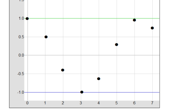
Understanding the Behavior of the Sequence aₙ = 2 + (-1)ⁿ/n
The sequence defined by aₙ = 2 + (-1)ⁿ/n exhibits an oscillatory behavior, but with a pattern that approaches a limit as n increases.
1. Analyzing the Behavior
The sequence alternates between two expressions depending on whether n is even or odd:
For even values of n, (-1)ⁿ = 1, so the term aₙ = 2 + 1/n.
For odd values of n, (-1)ⁿ = -1, so the term aₙ = 2 – 1/n.
As n increases, both expressions approach 2, so the sequence oscillates but also approaches 2.
2. List of Values
n=1: a₁ = 2 – 1/1 = 1
n=2: a₂ = 2 + 1/2 = 2.5
n=3: a₃ = 2 – 1/3 ≈ 1.6667…
n=4: a₄ = 2 + 1/4 = 2.25
n=5: a₅ = 2 – 1/5 = 1.8
…
3. Visualization Suggestion
To mentally visualize the behavior of the sequence, imagine a wave pattern that alternates between two levels but gradually gets closer to the horizontal line y = 2 as n increases. This captures both the oscillatory nature and the convergence of the sequence.
4. Conclusion
The sequence aₙ = 2 + (-1)ⁿ/n oscillates between two expressions but also approaches 2 as n increases. This behavior can be visualized as a wave pattern that gradually flattens, reflecting the alternating nature and convergence of the sequence.
Understanding the Behavior of the Sequence aₙ = (1 – n)/(3 + n)
The sequence defined by aₙ = (1 – n)/(3 + n) can be analyzed by looking at the expression, calculating terms, and taking the limit as n approaches infinity.
1. List of Values
n=1: a₁ = (1 – 1)/(3 + 1) = 0
n=2: a₂ = (1 – 2)/(3 + 2) = -0.2
n=3: a₃ = (1 – 3)/(3 + 3) = -0.3333…
n=4: a₄ = (1 – 4)/(3 + 4) ≈ -0.4286
n=5: a₅ = (1 – 5)/(3 + 5) = -0.5
2. Taking the Limit
To find the limit of the sequence as n approaches infinity, we can analyze the expression:
As n grows, the terms 1 and 3 become insignificant compared to -n and n, so we can consider the expression:
\( \lim_{n \to \infty} \frac{-n}{n} = -1 \)
3. Conclusion
The sequence aₙ = (1 – n)/(3 + n) decreases and approaches -1 as n increases. The pattern of the sequence and the simple limit calculation confirm this behavior.
As n becomes very large, the denominator grows much faster than the numerator, causing the fraction to approach 0:
lim (n → ∞) 1 / (4n² + 2n) = 0
This step confirms that the sequence gets arbitrarily close to 0 as n gets larger.
3. Conclusion
Since the limit of the sequence is 0, the sequence converges, and the limit is 0. This investigation has taken us through the process of simplifying a complex expression, understanding its behavior, and determining its convergence. It illustrates the power of mathematical analysis in understanding sequences and their properties.
Investigating the Convergence of the Sequence \( aₙ = n^{1/n} \)
We are investigating the convergence of a sequence defined by the expression \( aₙ = n^{1/n} \). We’ll break down the process into clear steps.
1. Understanding the Expression
The expression \( aₙ = n^{1/n} \) represents the nth root of n. As n increases, we are taking higher and higher roots of larger and larger numbers. We want to understand how this behaves as n approaches infinity.
2. Relating the Expression to the Exponential Function
We can rewrite any expression of the form \( x^y \) as \( e^{y \ln x} \). Applying this to our expression, we have:
\( aₙ = n^{1/n} = e^{(1/n) \ln n} \)
This step helps us relate the original expression to the exponential function, which has well-known properties and behavior.
3. Finding the Limit
To find the limit of the sequence as n approaches infinity, we can now work with the equivalent expression:
\( \lim_{n \to ∞} e^{(1/n) \ln n} \)
Since the exponential function is continuous, we can move the limit inside:
By applying L’Hôpital’s rule to the expression inside the limit, we find:
\( \lim_{n \to ∞} (1/n) \ln n = 0 \)
So the original limit becomes:
\( \lim_{n \to ∞} n^{1/n} = e^0 = 1 \)
4. Conclusion
The sequence \( aₙ = n^{1/n} \) converges to 1 as n approaches infinity. This result is a fascinating insight into the behavior of taking roots of increasing numbers. It shows that as we take higher and higher roots of larger and larger numbers, the values approach 1.
Investigating the Convergence of the Sequence \( aₙ = e^{-1/\sqrt{n}} \)
We are investigating the convergence of a sequence defined by the expression \( aₙ = e^{-1/\sqrt{n}} \). We’ll break down the process into clear steps.
1. Understanding the Expression
The expression \( aₙ = e^{-1/\sqrt{n}} \) represents the exponential function with a negative reciprocal of the square root of n in the exponent. As n increases, the exponent approaches 0, and we want to understand how this behaves as n approaches infinity.
2. Finding the Limit
To find the limit of the sequence as n approaches infinity, we can analyze the behavior of the exponent:
\( \lim_{n \to ∞} (-1/\sqrt{n}) = 0 \)
Since the exponential function is continuous, we can apply the limit to the entire expression:
\( \lim_{n \to ∞} e^{-1/\sqrt{n}} = e^0 = 1 \)
3. Conclusion
The sequence \( aₙ = e^{-1/\sqrt{n}} \) converges to 1 as n approaches infinity. This result provides insight into the behavior of the exponential function with a variable exponent that approaches 0. It illustrates how the exponential function behaves with complex expressions in the exponent and confirms the convergence of the sequence to 1.
Investigating the Convergence of the Sequence \( aₙ = \frac{{\ln(n)}}{{\ln(2n)}} \)
We are investigating the convergence of a sequence defined by the expression \( aₙ = \frac{{\ln(n)}}{{\ln(2n)}} \). We’ll break down the process into clear steps.
1. Understanding the Expression
The expression \( aₙ = \frac{{\ln(n)}}{{\ln(2n)}} \) represents the ratio of the natural logarithm of n to the natural logarithm of 2n. As n increases, both the numerator and denominator grow, and we want to understand how this behaves as n approaches infinity.
2. Finding the Limit
To find the limit of the sequence as n approaches infinity, we can use the properties of logarithms and simplify the expression:
The sequence \( aₙ = \frac{{\ln(n)}}{{\ln(2n)}} \) converges to 1 as n approaches infinity. This result provides insight into the behavior of the ratio of logarithms of increasing numbers. It illustrates how the natural logarithm function behaves with complex expressions and confirms the convergence of the sequence to 1.
Investigating the Convergence of the Sequence aₙ = arctan(ln(n))
We are investigating the convergence of a sequence defined by the expression aₙ = arctan(ln(n)). We’ll break down the process into clear steps.
1. Understanding the Expression
The expression aₙ = arctan(ln(n)) represents the arctangent of the natural logarithm of n. As n increases, the natural logarithm of n grows, and we want to understand how the arctangent behaves as n approaches infinity.
2. Finding the Limit
To find the limit of the sequence as n approaches infinity, we can analyze the behavior of the natural logarithm of n:
lim (n → ∞) ln(n) = ∞
Now, we can apply the arctangent function to this limit:
lim (n → ∞) arctan(ln(n)) = arctan(∞)
Since the arctangent function has a horizontal asymptote at π/2, the limit becomes:
The sequence aₙ = arctan(ln(n)) converges to π/2 as n approaches infinity. This result provides insight into the behavior of the arctangent function applied to the natural logarithm of increasing numbers. It illustrates how the arctangent function behaves with complex expressions and confirms the convergence of the sequence to π/2.
A recurrence relation is a mathematical expression that defines a sequence in terms of previous terms in the sequence. It’s like a recipe that tells you how to build the sequence step by step, using the values that you’ve already computed.
1. Definition
A recurrence relation for a sequence {aₙ} is an equation that expresses aₙ in terms of one or more of the previous terms aₙ₋₁, aₙ₋₂, … An initial condition is usually provided to start the sequence.
For example, the famous Fibonacci sequence is defined by the recurrence relation:
aₙ = aₙ₋₁ + aₙ₋₂ with initial conditions a₀ = 0 and a₁ = 1.
2. Intuitions
Recurrence relations can be thought of as a set of instructions or a process for building a sequence. They capture the pattern or rule that governs the sequence, allowing you to generate as many terms as you want, provided you know the initial conditions.
Imagine building a tower of blocks, where each block’s size is determined by the sizes of the previous two blocks. A recurrence relation is like the rule that tells you how to choose each block’s size based on the previous ones.
3. Benefits
Recurrence relations have several benefits in mathematics and other fields:
Pattern Recognition: They capture the underlying pattern or structure of a sequence, making it easier to understand and analyze.
Computational Efficiency: They provide an algorithmic way to compute the terms of a sequence, which can be implemented in computer programs.
Problem Solving: They are used to solve various problems in mathematics, computer science, engineering, and other disciplines, such as modeling growth, predicting outcomes, and analyzing algorithms.
Mathematical Analysis: They allow for the study of the properties of sequences, such as convergence, divergence, and behavior in the long term.
In summary, recurrence relations are a powerful tool for defining, understanding, and working with sequences. They provide a systematic way to generate the terms of a sequence and offer insights into the sequence’s behavior and properties.
Example of a Recurrence Relation
Let’s explore a simple recurrence relation to understand how it defines a sequence. We’ll use the following recurrence relation:
aₙ = 2 * aₙ₋₁ + 1
with the initial condition a₀ = 0.
1. Understanding the Relation
This recurrence relation tells us that each term in the sequence is twice the previous term plus 1. Starting with a₀ = 0, we can use this rule to find the next terms in the sequence.
2. Generating the Sequence
Using the recurrence relation, we can generate the first few terms of the sequence:
a₀ = 0 (initial condition)
a₁ = 2 * a₀ + 1 = 2 * 0 + 1 = 1
a₂ = 2 * a₁ + 1 = 2 * 1 + 1 = 3
a₃ = 2 * a₂ + 1 = 2 * 3 + 1 = 7
a₄ = 2 * a₃ + 1 = 2 * 7 + 1 = 15
3. Benefits and Insights
This simple example illustrates how a recurrence relation provides a systematic way to generate the terms of a sequence. It captures the pattern of the sequence and allows us to compute as many terms as we want, starting from the initial condition.
Recurrence relations like this one are used in various fields to model growth, analyze algorithms, and solve mathematical problems.
In summary, this example shows how a recurrence relation defines a sequence and provides insights into its behavior. It’s a powerful tool for understanding and working with sequences in mathematics and beyond.
Level 2 Example of a Recurrence Relation
Let’s explore a more complex recurrence relation that involves two previous terms. We’ll use the following recurrence relation:
aₙ = aₙ₋₁ + 2 * aₙ₋₂ + 3
with the initial conditions a₀ = 1 and a₁ = 2.
1. Understanding the Relation
This recurrence relation tells us that each term in the sequence is the sum of the previous term, twice the term before that, and 3. It’s a bit more complex than the previous example and requires two initial conditions to start the sequence.
2. Generating the Sequence
Using the recurrence relation, we can generate the first few terms of the sequence:
a₀ = 1 (initial condition)
a₁ = 2 (initial condition)
a₂ = a₁ + 2 * a₀ + 3 = 2 + 2 * 1 + 3 = 7
a₃ = a₂ + 2 * a₁ + 3 = 7 + 2 * 2 + 3 = 16
a₄ = a₃ + 2 * a₂ + 3 = 16 + 2 * 7 + 3 = 33
3. Insights and Applications
This example illustrates how recurrence relations can define more complex patterns in sequences. The relation captures the underlying structure of the sequence, allowing us to generate terms systematically.
Such recurrence relations are used in various applications, including financial modeling, computer algorithms, and mathematical problem-solving. They provide a way to describe complex behaviors and patterns in a concise mathematical form.
In summary, this Level 2 example shows how a more complex recurrence relation defines a sequence and offers insights into its behavior. It demonstrates the power and flexibility of recurrence relations in understanding and working with sequences.
Finding the Limit of a Sequence Defined by a Recurrence Relation
Let’s explore a simple recurrence relation and find the limit of the sequence it defines. We’ll use the following recurrence relation:
aₙ = 1/2 * aₙ₋₁
with the initial condition a₀ = 1.
1. Understanding the Relation
This recurrence relation tells us that each term in the sequence is half the previous term. It’s a simple relation that will help us understand how to find the limit of a sequence defined by a recurrence relation.
2. Generating the Sequence
Using the recurrence relation, we can generate the first few terms of the sequence:
a₀ = 1 (initial condition)
a₁ = 1/2 * a₀ = 1/2
a₂ = 1/2 * a₁ = 1/4
a₃ = 1/2 * a₂ = 1/8
a₄ = 1/2 * a₃ = 1/16
3. Finding the Limit
We can see that the terms of the sequence are getting smaller and smaller, approaching 0. Since each term is half the previous term, the sequence will continue to get closer to 0 without ever reaching it.
Mathematically, we can express this by saying that the limit of the sequence as n approaches infinity is 0:
lim (n → ∞) aₙ = 0
4. Insights and Understanding
This example illustrates how a simple recurrence relation can define a sequence whose behavior is easy to understand. By examining the pattern of the sequence, we can determine its limit and gain insights into the behavior of the sequence as it progresses.
Understanding the limits of sequences is fundamental in calculus, analysis, and various applications in science and engineering. It helps us understand the long-term behavior of sequences and functions.
In summary, this example shows how to find the limit of a sequence defined by a recurrence relation. It provides a clear and instructive demonstration of the concept, suitable for those learning about sequences and limits.
Finding the Limit of a More Complex Sequence Defined by a Recurrence Relation
Let’s explore a more intricate recurrence relation and find the limit of the sequence it defines. We’ll use the following recurrence relation:
aₙ = (aₙ₋₁ + 1) / 2
with the initial condition a₀ = 1.
1. Understanding the Relation
This recurrence relation tells us that each term in the sequence is the average of the previous term and 1. It’s a more complex relation that will help us delve deeper into finding the limit of a sequence defined by a recurrence relation.
2. Generating the Sequence
Using the recurrence relation, we can generate the first few terms of the sequence:
a₀ = 1 (initial condition)
a₁ = (a₀ + 1) / 2 = 1
a₂ = (a₁ + 1) / 2 = 1
a₃ = (a₂ + 1) / 2 = 1
a₄ = (a₃ + 1) / 2 = 1
3. Finding the Limit
We can see that after the first term, the sequence becomes constant, and all subsequent terms are equal to 1. Since the sequence is constant, it converges to the value of any of its terms.
Mathematically, we can express this by saying that the limit of the sequence as n approaches infinity is 1:
lim (n → ∞) aₙ = 1
4. Insights and Understanding
This example illustrates how a more complex recurrence relation can define a sequence whose behavior might not be immediately obvious. By carefully examining the pattern of the sequence and applying the recurrence relation, we can determine its limit.
Understanding the limits of sequences is essential in various mathematical fields, including calculus and real analysis. It provides insights into the long-term behavior of sequences and functions and is a foundational concept in mathematics.
In summary, this more complex example shows how to find the limit of a sequence defined by a recurrence relation. It provides a deeper understanding of the concept and demonstrates the process in a more intricate scenario.
The Completeness of the Real Numbers (ℝ) and Convergence of Sequences
The completeness of the real numbers ensures that there are no “gaps” or “holes” in the number line. It plays a crucial role in understanding the convergence of sequences. Here’s how:
1. Least Upper Bound (LUB) Property
The Least Upper Bound Property states that any non-empty set of real numbers that is bounded above has a least upper bound (LUB), also known as the supremum. Similarly, any non-empty set of real numbers that is bounded below has a greatest lower bound (GLB), also known as the infimum.
This property is directly related to the convergence of sequences. If you have a monotonic increasing sequence that is bounded above, the LUB of the set of terms in the sequence is the limit to which the sequence converges. Similarly, if you have a monotonic decreasing sequence that is bounded below, the GLB of the set of terms in the sequence is the limit to which the sequence converges.
Visualizing Completeness with a Highlighter and Number Line
Imagine you have a highlighter and a number line that represents the real numbers. You can think of completeness as the ability to highlight the entire number line without missing any points.
If you were to highlight only the rational numbers, you would miss the irrational numbers, leaving “gaps” in the number line. But with the real numbers, every point on the number line corresponds to a real number, so you can highlight the entire line without missing anything.
In terms of sequences, you can think of a converging sequence as a series of points on the number line that get closer and closer to a specific value. Because of completeness, you know that this value is a real number, and there’s no “gap” where the sequence is heading.
Significance of Completeness in Convergence
The completeness property ensures that every bounded, monotonic sequence in the real numbers must converge to a real number. This is a fundamental result known as the Monotonic Sequence Theorem.
Without completeness, we could have sequences that seem to approach a limit but don’t actually converge to any real number. Completeness fills in the “gaps” and ensures that such situations don’t occur in the real numbers.
In summary, the completeness of the real numbers is essential for understanding the convergence of sequences. It guarantees that bounded, monotonic sequences have a limit in the real numbers, and it can be visualized as the ability to highlight the entire number line without missing any points. This property underpins many of the results and methods used in mathematical analysis, calculus, and beyond.
Example of Completeness for a Convergent Sequence: 1/n
Consider the sequence defined by 1/n, where n is a positive integer. This sequence converges to 0 in the real numbers. But what if 0 were not included in our number system? Let’s explore this scenario:
Sequence: 1/n
The terms of this sequence are:
1/1 = 1
1/2 = 0.5
1/3 ≈ 0.333
1/4 = 0.25
…
Convergence to 0 in the Real Numbers
In the real numbers, the sequence 1/n converges to 0. As n gets larger, the value of 1/n gets closer and closer to 0.
Hypothetical Scenario: 0 Not Included
Now, imagine a hypothetical number system where 0 is not included. In this system, the sequence 1/n would not have a limit, because the value it’s approaching (0) does not exist in the system. The sequence would continue to get closer to a “gap” where 0 should be, but it would never actually converge.
Role of Completeness
The completeness of the real numbers ensures that every point on the number line, including 0, corresponds to a real number. This allows the sequence 1/n to converge to 0. Without completeness, and without the inclusion of 0, the sequence would not have a limit in the system.
In summary, this example illustrates how the completeness of the real numbers, including the inclusion of 0, ensures that the sequence 1/n converges to 0. Without completeness, and without 0, the sequence would not converge, highlighting the importance of completeness in understanding the behavior of sequences.
Monotonic Sequence Theorem
The Monotonic Sequence Theorem states that every bounded, monotonic sequence in the real numbers is convergent. Here’s how the proof can be understood with both rigor and intuition:
1. Definitions
A sequence is called monotonic if it is either non-decreasing (each term is greater than or equal to the previous term) or non-increasing (each term is less than or equal to the previous term). A sequence is bounded if there is a real number that is an upper bound for all the terms (for a non-decreasing sequence) or a lower bound for all the terms (for a non-increasing sequence).
2. Intuitive Understanding
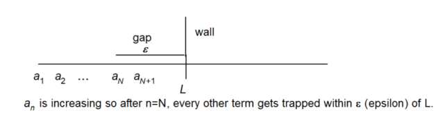
Imagine a number line, and think of a monotonic sequence as a series of points on that line that are either moving steadily to the right (non-decreasing) or to the left (non-increasing). If there’s a “wall” (an upper or lower bound) that the points can’t pass, then the points must eventually get closer and closer to a specific value, and the sequence must converge.
3. Rigorous Proof
Existence of the Least Upper Bound (LUB): Since the sequence is bounded above, the set of its terms has an upper bound. By the completeness of the real numbers, this set has a least upper bound, say L.
Show that L is the Limit:
We want to show that for any ε > 0, there exists an N such that for all n ≥ N, |aₙ – L| < ε.
Since L is the least upper bound, any number smaller than L, like L – ε, cannot be an upper bound for the sequence. This means that there must be some term in the sequence, say aₙ with index N, that is greater than L – ε.
Since the sequence is non-decreasing, all subsequent terms (for n > N) must also be greater than L – ε. And since L is an upper bound, all terms must be less than or equal to L. Therefore, for all n ≥ N, the difference between aₙ and L is less than ε, so |aₙ – L| < ε.
This shows that the sequence gets arbitrarily close to L as n gets larger, so L is the limit of the sequence.
Conclusion: The sequence converges to L.
In summary, the Monotonic Sequence Theorem can be understood both intuitively, as a series of points on a number line approaching a “wall,” and rigorously, using the completeness of the real numbers and the definition of convergence. It ensures that every bounded, monotonic sequence in the real numbers must converge, providing a powerful tool for understanding the behavior of sequences.
Visualizing the Proof of the Monotonic Sequence Theorem
The Monotonic Sequence Theorem is a foundational result in real analysis. Here’s how you can visualize the key parts of the proof:
1. Existence of the Least Upper Bound (LUB):
Imagine the terms of the sequence as points on a number line. Since the sequence is bounded above, there is a “wall” or barrier (an upper bound) that the terms cannot pass. The least upper bound (LUB) is the closest point to the terms that still acts as a barrier. It’s like the sequence is trying to reach this point but can never quite get there.
By the completeness of the real numbers, this LUB must exist, and we call it L.
2. Show that L is the Limit:
Now, we want to show that the sequence actually converges to L. To visualize this:
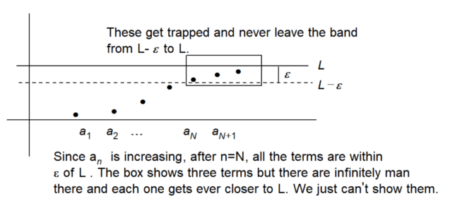
Think of ε as a small gap or buffer around L. The sequence must get within this gap as n gets larger.
Since L is the least upper bound, any number smaller than L, like L – ε, cannot be an upper bound. So there must be some term in the sequence that enters this gap.
Since the sequence is non-decreasing, all subsequent terms must also enter this gap and stay there. They can’t go past L because L is an upper bound, but they must be greater than L – ε.
This means that the sequence gets closer and closer to L, squeezing into the gap around L, and thus converging to L.
3. Conclusion:
The sequence converges to L. You can think of the sequence as a series of points on a number line, steadily approaching L but never going past it. The completeness of the real numbers ensures that L exists, and the non-decreasing nature of the sequence ensures that it converges to L.
This visualization helps to make the abstract concepts in the proof more concrete and relatable, providing a mental picture of what’s happening in the proof.
A sequence (aₙ) is said to be bounded above if there exists a real number M such that aₙ ≤ M for all n ∈ ℕ. In other words, no term in the sequence is greater than M, and M is called an upper bound of the sequence.
Bounded Below
A sequence (aₙ) is said to be bounded below if there exists a real number m such that aₙ ≥ m for all n ∈ ℕ. In other words, no term in the sequence is less than m, and m is called a lower bound of the sequence.
Bounded
A sequence is simply called bounded if it is both bounded above and bounded below. This means that there exist real numbers M and m such that m ≤ aₙ ≤ M for all n ∈ ℕ. In this case, the sequence is confined within a fixed range, and no term can go to infinity or negative infinity.
These concepts are fundamental in real analysis and are used to study the properties of sequences and their convergence behavior.
Simple Examples: Bounded Above
A sequence that is bounded above has a limit to how high the numbers can go. For example, consider the sequence: 2, 4, 6, 8, 10. No number in this sequence is greater than 10, so we say it’s bounded above by 10.
Bounded Below
A sequence that is bounded below has a limit to how low the numbers can go. For example, consider the sequence: 5, 3, 4, 5, 6. No number in this sequence is less than 3, so we say it’s bounded below by 3.
Bounded
If a sequence is both bounded above and below, the numbers are trapped within a specific range. For example, consider the sequence: 7, 8, 7, 8, 7. The numbers in this sequence are never greater than 8 and never less than 7, so we say it’s bounded by 7 and 8.
Understanding whether a sequence is bounded helps mathematicians and scientists analyze patterns and make predictions. It’s like knowing the minimum and maximum temperatures for the day; you know how to dress because you know it won’t get too hot or too cold.
Bounded Above
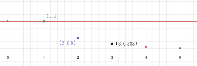
A sequence that is bounded above has a limit to how high the numbers can go. Consider the sequence defined by the expression aₙ = 1/n, where n is a natural number starting from 1 (1, 2, 3, …).
This sequence looks like: 1/1, 1/2, 1/3, 1/4, 1/5, …
In this sequence, as n gets larger, the value of 1/n gets smaller. However, no matter how large n gets, the value of 1/n will never be greater than 1. So, we can say that this sequence is bounded above by 1.
This means that all the numbers in the sequence are less than or equal to 1, and 1 is the upper bound of the sequence.
In the graph created in Desmos, the horizontal line y = 1 represents the upper bound for the sequence defined by aₙ = 1/n. Alongside this line, individual points are plotted for x = 1, x = 2, x = 3, x = 4, and x = 5, corresponding to the values (1, 1/1), (2, 1/2), (3, 1/3), (4, 1/4), and (5, 1/5) respectively. These points illustrate the values of the sequence and visually demonstrate how the terms of the sequence approach 0 as n increases, yet never exceed the value of 1. The graph effectively captures the idea that the sequence is bounded above by 1, providing a clear and intuitive visual representation of this mathematical concept.
Bounded Above and Increasing
Consider the sequence defined by the expression aₙ = n / (n + 1), where n is a natural number starting from 1 (1, 2, 3, …).
This sequence looks like: 1/2, 2/3, 3/4, 4/5, 5/6, …
In this sequence, as n gets larger, both the numerator and the denominator increase, but the value of n / (n + 1) gets closer and closer to 1. So, we can say that this sequence is bounded above by 1.
This means that all the numbers in the sequence are less than or equal to 1, and 1 is the upper bound of the sequence. Additionally, since each term is greater than the previous term, the sequence is increasing.
If you were to graph this sequence in Desmos, you would see the individual points for x = 1, x = 2, x = 3, x = 4, and x = 5, corresponding to the values (1, 1/2), (2, 2/3), (3, 3/4), (4, 4/5), and (5, 5/6) respectively, all lying below the horizontal line y = 1. This graph would visually demonstrate how the sequence is both bounded above by 1 and increasing.
An Upper Bound vs. The Upper Bound (Least Upper Bound)
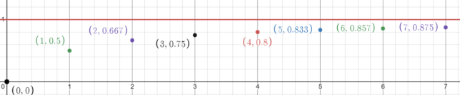
Consider the sequence defined by the expression aₙ = n / (n + 1), where n is a natural number starting from 1.
This sequence looks like: 1/2, 2/3, 3/4, 4/5, 5/6, …
An Upper Bound
“An upper bound” refers to any number that is greater than or equal to every term in the sequence. For example, the numbers 2, 1.5, and 1 are all upper bounds for this sequence.
However, 0.8 is not an upper bound, as there are values in the sequence, like 4/5 (0.8) and 5/6 (approximately 0.833), that are equal to or greater than 0.8.
Values in the sequence:
1/2 is less than 2, 1.5, 1, and 0.8
2/3 is less than 2, 1.5, 1, and 0.8
3/4 is less than 2, 1.5, 1, and 0.8
4/5 is equal to 0.8 and less than 2, 1.5, and 1
5/6 is greater than 0.8 and less than 2, 1.5, and 1
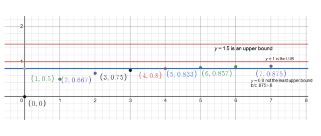
The Upper Bound (Least Upper Bound)
“The upper bound” or “the least upper bound” (LUB) refers to the smallest number that is an upper bound for the sequence. In this case, the LUB is 1. There is no number smaller than 1 that is greater than or equal to every term in the sequence.
Your graph shows the lines y = 0.8, y = 1.5, and y = 1. The line y = 1 represents the LUB, while y = 0.8 is not an upper bound as some terms in the sequence are greater than 0.8. The line y = 1.5 represents another upper bound but is not the LUB as it is not the smallest upper bound.
Values in the sequence compared to the LUB:
1/2 is less than 1 (the LUB)
2/3 is less than 1 (the LUB)
3/4 is less than 1 (the LUB)
4/5 is less than 1 (the LUB)
5/6 is less than 1 (the LUB)
This distinction between “an upper bound” and “the upper bound” helps us understand how sequences behave and provides insights into their properties and limits.
Monotonic Increasing and Monotonic Decreasing Sequences
Monotonic Increasing
A sequence is said to be monotonic increasing if each term is greater than or equal to the previous term. An example of a monotonic increasing sequence is aₙ = n.
Values in the sequence:
a₁ = 1
a₂ = 2
a₃ = 3
a₄ = 4
a₅ = 5
This sequence shows that each term is greater than the previous one: 1 < 2 < 3 < 4 < 5, and so on.
Monotonic Decreasing
A sequence is said to be monotonic decreasing if each term is less than or equal to the previous term. An example of a monotonic decreasing sequence is aₙ = 1 / n.
Values in the sequence:
a₁ = 1
a₂ = 1/2
a₃ = 1/3
a₄ = 1/4
a₅ = 1/5
This sequence shows that each term is less than the previous one: 1 > 1/2 > 1/3 > 1/4 > 1/5, and so on.
Understanding whether a sequence is monotonic increasing or decreasing can provide insights into its behavior, convergence, and other properties. Monotonic sequences are often encountered in mathematical analysis and have applications in various fields.
Monotonic Increasing vs. Increasing
Monotonic Increasing
A sequence is said to be monotonic increasing if each term is greater than or equal to the previous term. In other words, the sequence can stay the same or increase, but it cannot decrease. The key here is that the sequence is allowed to have consecutive terms that are equal.
Example of a monotonic increasing sequence: 1, 2, 2, 3, 3, 3, 4, 5, …
Strictly Increasing
A sequence is said to be strictly increasing if each term is strictly greater than the previous term. Unlike monotonic increasing, a strictly increasing sequence cannot have consecutive terms that are equal; each term must be greater than the one before it.
Example of a strictly increasing sequence: 1, 2, 3, 4, 5, …
Comparison
While both monotonic increasing and strictly increasing sequences involve terms that get larger, the key difference lies in how they handle equality:
Monotonic Increasing: Allows consecutive terms to be equal (e.g., 2, 2, 3).
Strictly Increasing: Does not allow consecutive terms to be equal; each term must be greater than the previous one (e.g., 2, 3, 4).
It’s worth noting that all strictly increasing sequences are also monotonic increasing, but not all monotonic increasing sequences are strictly increasing.
Understanding these distinctions is important in mathematical analysis and other fields, as different properties and theorems may apply depending on whether a sequence is monotonic increasing or strictly increasing.
For what values of r is the sequence rⁿ convergent?
Answer:
The sequence rⁿ is convergent if and only if |r| < 1. Let's break down the cases to understand why:
For |r| < 1:
When the absolute value of r is less than 1, each term is multiplied by a fraction, making the terms get closer and closer to 0.
Example with r = 0.5: 0.5 × 0.5 = 0.25, 0.25 × 0.5 = 0.125, …
Example with r = -0.5: (-0.5) × (-0.5) = 0.25, 0.25 × (-0.5) = -0.125, …
For |r| = 1:
When the absolute value of r is exactly 1, the terms will either be constant or oscillate between two values.
Example with r = 1: 1 × 1 = 1, 1 × 1 = 1, …
Example with r = -1: (-1) × (-1) = 1, 1 × (-1) = -1, …
For |r| > 1:
When the absolute value of r is greater than 1, each term is multiplied by a number greater than 1, making the terms grow without bound.
Example with r = 2: 2 × 2 = 4, 4 × 2 = 8, 8 × 2 = 16, …
Example with r = -2: (-2) × (-2) = 4, 4 × (-2) = -8, 16 × (-2) = 16, …
Why r = 1 is the Breakpoint:
The value r = 1 is the natural breakpoint because it’s the boundary between the three distinct behaviors of the sequence.
Choosing other values like r = 2 or r = 0.5 as the breakpoint would not capture the essential differences in behavior.
This analysis helps us understand why the sequence rⁿ is convergent for |r| < 1 and divergent otherwise.
\[
\begin{align*}
\text{Convergence of } r^n =
\begin{cases}
\text{Converges to } 0 & \text{if } |r| < 1 \\
\text{Oscillates or is constant} & \text{if } |r| = 1 \\
\text{Diverges} & \text{if } |r| > 1
\end{cases}
\end{align*}
\]
Increasing Sequences
An increasing sequence is a sequence where each term is greater than or equal to the previous term. In mathematical terms, a sequence (aₙ) is increasing if aₙ₊₁ ≥ aₙ for all n.
Understanding the Subscripts:
The subscript n represents the position of a term in the sequence. For example, aₙ is the nth term, a₃ is the third term, and so on.
The subscript n+1 represents the next position after n. So if aₙ is the nth term, then aₙ₊₁ is the (n+1)th term, or the term immediately following aₙ.
Example:
Consider the sequence defined by aₙ = n². This sequence is increasing because:
aₙ = n² (the nth term)
aₙ₊₁ = (n+1)² (the (n+1)th term, or the term immediately after the nth term)
Since (n+1)² > n², we have aₙ₊₁ > aₙ for all n, so the sequence is increasing.
Here’s a comparison between consecutive terms:
a₁ (first term) = 1² = 1
a₂ (second term) = 2² = 4, a₂ > a₁
a₃ (third term) = 3² = 9, a₃ > a₂
…
In this example, the subscript n represents the position of the term, and n+1 represents the next position. By comparing the terms at these positions, we can see that the sequence is increasing.
Decreasing Sequences
A decreasing sequence is a sequence where each term is less than or equal to the previous term. In mathematical terms, a sequence (aₙ) is decreasing if aₙ₊₁ ≤ aₙ for all n.
Understanding the Subscripts:
The subscript n represents the position of a term in the sequence. For example, aₙ is the nth term, a₃ is the third term, and so on.
The subscript n+1 represents the next position after n. So if aₙ is the nth term, then aₙ₊₁ is the (n+1)th term, or the term immediately following aₙ.
Example:
Consider the sequence defined by aₙ = -n². This sequence is decreasing because:
aₙ = -n² (the nth term)
aₙ₊₁ = -(n+1)² (the (n+1)th term, or the term immediately after the nth term)
Since -(n+1)² < -n², we have aₙ₊₁ < aₙ for all n, so the sequence is decreasing.
Here’s a comparison between consecutive terms:
a₁ (first term) = -1² = -1
a₂ (second term) = -2² = -4, a₂ < a₁
a₃ (third term) = -3² = -9, a₃ < a₂
…
In this example, the subscript n represents the position of the term, and n+1 represents the next position. By comparing the terms at these positions, we can see that the sequence is decreasing.
The sequence defined by \( a_n = \frac{2}{n + 1} \) is decreasing. We can prove this by comparing consecutive terms:
\( a_n = \frac{2}{n + 1} \) (the nth term)
\( a_{n+1} = \frac{2}{(n + 1) + 1} = \frac{2}{n + 2} \) (the (n+1)th term, or the term immediately after the nth term)
Since \( \frac{2}{n + 1} > \frac{2}{n + 2} \), we have \( a_{n+1} < a_n \) for all \( n \geq 0 \), so the sequence is decreasing.
Explanation:
The denominator \( n + 1 \) in \( a_n \) represents the nth term’s denominator.
The denominator \( n + 2 \) in \( a_{n+1} \) represents the (n+1)th term’s denominator, which is one more than the nth term’s denominator.
Since the numerators are the same (2) and the denominators are increasing, the fractions are decreasing.
This example shows that the sequence \( \left\{ \frac{2}{n + 1} \right\} \) is decreasing, and it provides a clear understanding of how the terms were compared to reach this conclusion.
Step 2: Cross-multiply to eliminate fractions: \( n(n+1)^2 + n < n(n^2 + 1) + n^2 + 1 \)
Step 3: Expand both sides to simplify: \( n^3 + 2n^2 + n + n < n^3 + n^2 + n + n^2 + 1 \)
Step 4: Rearrange terms to isolate the inequality: \( 1 < n^2 + n \)
Step 5: This inequality \( 1 < n^2 + n \) has the same meaning as our original inequality but is simpler to understand. It clearly shows that the terms of the sequence are decreasing.
Since \( n > 1 \), we conclude that \( 1 < n^2 + n \), and the sequence is decreasing.
Conclusion: The sequence \( \left\{ \frac{n}{n^2 + 1} \right\} \) is decreasing as we have shown that consecutive terms are less than the previous ones. The simplified inequality \( 1 < n^2 + n \) helped us understand this more clearly.
Example: Decreasing Sequence \( \left\{ \frac{n}{n^2 + 1} \right\} \) Using the Function Version
We can analyze the sequence by considering the corresponding function and its derivative.
Define the Function
Consider the function \( f(x) = \frac{x}{x^2 + 1} \).
Find the Derivative
We’ll use the quotient rule to find the derivative:
The function is decreasing when \( f'(x) < 0 \), which occurs when \( x^2 > 1 \), i.e., \( x > 1 \) or \( x < -1 \).
The function is increasing when \( f'(x) > 0 \), which occurs when \( -1 < x < 1 \).
Conclusion for the Sequence
Since the derivative is negative for \( x > 1 \), the function is decreasing for those values of \( x \), and thus the sequence \( \left\{ \frac{n}{n^2 + 1} \right\} \) is decreasing for \( n > 1 \).